Introduction tutorial
In this tutorial we will perform handwriting recognition by training a multilayer perceptron (MLP) on the MNIST handwritten digit database.
The Task
MNIST is a dataset which consists of 70,000 handwritten digits. Each digit is a grayscale image of 28 by 28 pixels. Our task is to classify each of the images into one of the 10 categories representing the numbers from 0 to 9.
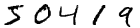
Sample MNIST digits
The Model
We will train a simple MLP with a single hidden layer that uses the rectifier activation function. Our output layer will consist of a softmax function with 10 units; one for each class. Mathematically speaking, our model is parametrized by \(\mathbf{\theta}\), defined as the weight matrices \(\mathbf{W}^{(1)}\) and \(\mathbf{W}^{(2)}\), and bias vectors \(\mathbf{b}^{(1)}\) and \(\mathbf{b}^{(2)}\). The rectifier activation function is defined as
and our softmax output function is defined as
Hence, our complete model is
Since the output of a softmax sums to 1, we can interpret it as a categorical probability distribution: \(f(\mathbf{x})_c = \hat p(y = c \mid \mathbf{x})\), where \(\mathbf{x}\) is the 784-dimensional (28 × 28) input and \(c \in \{0, ..., 9\}\) one of the 10 classes. We can train the parameters of our model by minimizing the negative log-likelihood i.e. the cross-entropy between our model’s output and the target distribution. This means we will minimize the sum of
(where \(\mathbf{1}\) is the indicator function) over all examples. We use stochastic gradient descent (SGD) on mini-batches for this.
Building the model
Blocks uses “bricks” to build models. Bricks are parametrized Theano operations. You can read more about it in the building with bricks tutorial.
Constructing the model with Blocks is very simple. We start by defining the input variable using Theano.
Tip
Want to follow along with the Python code? If you are using IPython, enable
the doctest mode using the special %doctest_mode command so that you
can copy-paste the examples below (including the >>> prompts) straight
into the IPython interpreter.
>>> from theano import tensor
>>> x = tensor.matrix('features')
Note that we picked the name 'features' for our input. This is important,
because the name needs to match the name of the data source we want to train on.
MNIST defines two data sources: 'features' and 'targets'.
For the sake of this tutorial, we will go through building an MLP the long way. For a much quicker way, skip right to the end of the next section. We begin with applying the linear transformations and activations.
We start by initializing bricks with certain parameters e.g. input_dim.
After initialization we can apply our bricks on Theano variables to build the model
we want. We’ll talk more about bricks in the next tutorial, Building with bricks.
>>> from blocks.bricks import Linear, Rectifier, Softmax
>>> input_to_hidden = Linear(name='input_to_hidden', input_dim=784, output_dim=100)
>>> h = Rectifier().apply(input_to_hidden.apply(x))
>>> hidden_to_output = Linear(name='hidden_to_output', input_dim=100, output_dim=10)
>>> y_hat = Softmax().apply(hidden_to_output.apply(h))
Loss function and regularization
Now that we have built our model, let’s define the cost to minimize. For this, we will need the Theano variable representing the target labels.
>>> y = tensor.lmatrix('targets')
>>> from blocks.bricks.cost import CategoricalCrossEntropy
>>> cost = CategoricalCrossEntropy().apply(y.flatten(), y_hat)
To reduce the risk of overfitting, we can penalize excessive values of the parameters by adding a \(L2\)-regularization term (also known as weight decay) to the objective function:
To get the weights from our model, we will use Blocks’ annotation features (read more about them in the Managing the computation graph tutorial).
>>> from blocks.roles import WEIGHT
>>> from blocks.graph import ComputationGraph
>>> from blocks.filter import VariableFilter
>>> cg = ComputationGraph(cost)
>>> W1, W2 = VariableFilter(roles=[WEIGHT])(cg.variables)
>>> cost = cost + 0.005 * (W1 ** 2).sum() + 0.005 * (W2 ** 2).sum()
>>> cost.name = 'cost_with_regularization'
Note
Note that we explicitly gave our variable a name. We do this so that when we monitor the performance of our model, the progress monitor will know what name to report in the logs.
Here we set \(\lambda_1 = \lambda_2 = 0.005\). And that’s it! We now have the final objective function we want to optimize.
But creating a simple MLP this way is rather cumbersome. In practice, we would
have used the MLP class instead.
>>> from blocks.bricks import MLP
>>> mlp = MLP(activations=[Rectifier(), Softmax()], dims=[784, 100, 10]).apply(x)
Initializing the parameters
When we constructed the Linear bricks to build our
model, they automatically allocated Theano shared variables to store their
parameters in. All of these parameters were initially set to NaN. Before
we start training our network, we will want to initialize these parameters
by sampling them from a particular probability distribution. Bricks can do this
for you.
>>> from blocks.initialization import IsotropicGaussian, Constant
>>> input_to_hidden.weights_init = hidden_to_output.weights_init = IsotropicGaussian(0.01)
>>> input_to_hidden.biases_init = hidden_to_output.biases_init = Constant(0)
>>> input_to_hidden.initialize()
>>> hidden_to_output.initialize()
We have now initialized our weight matrices with entries drawn from a normal distribution with a standard deviation of 0.01.
>>> W1.get_value()
        array([[ 0.01624345, -0.00611756, -0.00528172, ...,  0.00043597, ...
Training your model
Besides helping you build models, Blocks also provides the main other features needed to train a model. It has a set of training algorithms (like SGD), an interface to datasets, and a training loop that allows you to monitor and control the training process.
We want to train our model on the training set of MNIST. We load the data using the Fuel framework. Have a look at this tutorial to get started.
After having configured Fuel, you can load the dataset.
>>> from fuel.datasets import MNIST
>>> mnist = MNIST(("train",))
Datasets only provide an interface to the data. For actual training, we will need to iterate over the data in minibatches. This is done by initiating a data stream which makes use of a particular iteration scheme. We will use an iteration scheme that iterates over our MNIST examples sequentially in batches of size 256.
>>> from fuel.streams import DataStream
>>> from fuel.schemes import SequentialScheme
>>> from fuel.transformers import Flatten
>>> data_stream = Flatten(DataStream.default_stream(
...     mnist,
...     iteration_scheme=SequentialScheme(mnist.num_examples, batch_size=256)))
The training algorithm we will use is straightforward SGD with a fixed learning rate.
>>> from blocks.algorithms import GradientDescent, Scale
>>> algorithm = GradientDescent(cost=cost, parameters=cg.parameters,
...                             step_rule=Scale(learning_rate=0.1))
During training we will want to monitor the performance of our model on a separate set of examples. Let’s create a new data stream for that.
>>> mnist_test = MNIST(("test",))
>>> data_stream_test = Flatten(DataStream.default_stream(
...     mnist_test,
...     iteration_scheme=SequentialScheme(
...         mnist_test.num_examples, batch_size=1024)))
In order to monitor our performance on this data stream during training, we need
to use one of Blocks’ extensions, namely the DataStreamMonitoring
extension.
>>> from blocks.extensions.monitoring import DataStreamMonitoring
>>> monitor = DataStreamMonitoring(
...     variables=[cost], data_stream=data_stream_test, prefix="test")
We can now use the MainLoop to combine all the different
bits and pieces. We use two more extensions to make our training stop after
a single epoch and to make sure that our progress is printed.
>>> from blocks.main_loop import MainLoop
>>> from blocks.extensions import FinishAfter, Printing
>>> main_loop = MainLoop(data_stream=data_stream, algorithm=algorithm,
...                      extensions=[monitor, FinishAfter(after_n_epochs=1), Printing()])
>>> main_loop.run()

-------------------------------------------------------------------------------
BEFORE FIRST EPOCH
-------------------------------------------------------------------------------
Training status:
     epochs_done: 0
     iterations_done: 0
Log records from the iteration 0:
     test_cost_with_regularization: 2.34244632721


-------------------------------------------------------------------------------
AFTER ANOTHER EPOCH
-------------------------------------------------------------------------------
Training status:
     epochs_done: 1
     iterations_done: 235
Log records from the iteration 235:
     test_cost_with_regularization: 0.664899230003
     training_finish_requested: True


-------------------------------------------------------------------------------
TRAINING HAS BEEN FINISHED:
-------------------------------------------------------------------------------
Training status:
     epochs_done: 1
     iterations_done: 235
Log records from the iteration 235:
     test_cost_with_regularization: 0.664899230003
     training_finish_requested: True
     training_finished: True